 I’ve got a crazy idea for a new extension to my HDMI Light project… I’ll save the details for another day, but it will only work if I can accurately find the position of many small objects. I’d considered a few options, but as I’ve got an HTC Vive VR system, I thought I might be able to use its tracking system to do the locating.
This has turned out to be a way bigger project than I first expected, and as I tend to ramble a bit at the best of times, this has turned into my longest write-up ever, so before I start, here’s a quick summary:
- 4 sensors, 30 positions/s each
- Totally standalone, works out lighthouse positions for itself
- No configuration, apply power… get position data
- Accounts for gravity direction using accelerometer data from lighthouses
- Output sent via USB serial and/or UART
- Running on a 20MHz AVR
- Github here
The Vive Lighthouse System
Lighthouse animation by rvdm88
As shown in the animation above (click to see rvdm88’s full version on YouTube), this is achieved by the precise timing of a sequence of floodlight flashes and laser lines that sweep across the room. The core idea is that a lighthouse can signal the start of a sweep by lighting up the whole room with a synchronisation pulse from the floodlight, then by measuring the amount of time that passes before it is hit by the laser line sweep, a photo-diode can calculate its angle from the center line of the lighthouse.
Knowing the position of the lighthouses and the angles from the lighthouses to the photo-diode, it only takes basic trigonometry to triangulate the position of the photo-diode.
Each lighthouse sweeps the room with two perpendicular laser lines, one after the other, and the two lighthouses take turns to do their pair of sweeps, giving a total of four sweeps before the pattern repeats.
Each individual sweep takes a total of 8333uS, and they all start with a synchronisation pulse from both lighthouses, first a sync pulse from the master lighthouse, then a sync pulse from the slave 400uS later, then the sweep of the laser line. The time is directly related to the angle of the laser line, the full 8333uS represents 180 degrees, and straight ahead is centered at 4000 uS.
Each sweep cycle within the sequence of four contains the following pulses:
| Start Time | Length | Description |
|---|---|---|
| 0 uS | 62-135 uS | Master Sync Pulse |
| 400 uS | 62-135 uS | Slave Sync Pulse |
| 1222-6777 uS | ~10 uS | Laser Line Sweep |
| 8333 uS | End Of Cycle |
The photo-diode knows which lighthouse a sweep is coming from, and whether it is a horizontal or vertical sweep because the synchronisation flashes before each sweep are different lengths. The lengths of the synchronisation pulses encode three pieces of information:
- Whether this lighthouse will skip this sweep to let the other lighthouse take a turn
- One data bit that can be used, along with the bits from many other cycles, to build an OOTX message that contains several pieces of data about the lighthouse
- The axis of the following sweep
The pulse length encoding is as follows:
| Will Skip | Data Bit | Axis | Length |
|---|---|---|---|
| 0 | 0 | 0 | 62.5 uS |
| 0 | 0 | 1 | 72.9 uS |
| 0 | 1 | 0 | 83.3 uS |
| 0 | 1 | 1 | 93.8 uS |
| 1 | 0 | 0 | 104 uS |
| 1 | 0 | 1 | 115 uS |
| 1 | 1 | 0 | 125 uS |
| 1 | 1 | 1 | 135 uS |
There is one problem with this system… it only works if we know the precise position and orientation of the base stations. Once we know this then we can determine position with our single photo-diode, but how do we measure it in the first place? I’ll save the details for later… for now I’ll just say what I knew when I started… apparently, if we have four photo-diodes with known spacing then we can calculate the position and orientation of the base stations.
Choosing A Microcontroller
JTAG2UPDI Programmer
I’m most familiar with AVRs, and knowing that I was going to need to accurately timestamp the rising and falling edges of pulses from four separate sensors, I just looked at this table of AVR peripherals and ordered the ATmega with the most 16-bit timers… the ATmega3209.
I hadn’t been keeping up with changes to the AVR product line, the last time I’d ordered any was before Microchip bought them out, so I didn’t realise that this was a brand new part with significantly different peripherals. Or that I was going to need a new compiler and a new programmer. Which was lucky because I probably wouldn’t have ordered it if I had, but it’s actually a really nice part. The relevant spec’s include:
- 8-bit CPU with AVR instruction set
- 20MHz oscillator built in
- 4KB SRAM, 32KB Flash
- 5x 16-bit timers, 4 of which have input capture
- 4x USART
- Configurable pin-out via new event routing system
The first downside was that my compiler knew nothing about it, but that was fixed relatively quickly by downloading an updated compiler, which still didn’t know anything about it, and then an updated parts database.
The next problem was my AVRISP mkII programmer was also useless. These new parts use a single wire (or two if you count ground) programming system called Unified Program & Debug Interface (UPDI). Luckily I found the jtag2updi project on github, which allowed me to turn an ATmega88 into a programmer that works with avrdude via a USB serial interface.
With those two initial problems out of the way I was up and running again with only one day lost. There was one other problem that wouldn’t reveal itself until later though… That shiny new parts database I downloaded contains a bad crtatmega3209.o file. The interrupt vector table in that file is too short!
I didn’t discover this until I tried to use the fourth TCB timer’s interrupts. Every time I tried to use them, my code died, just like it would if I’d forgotten to declare an interrupt handler. Looking at the disassembly of the generated code quickly revealed the short interrupt vector table, but it took a bit longer to work out why it was happening. Luckily though, once I’d found the offending file, copying the equivalent file from the atmega4809 part seemed to work.
Amplifying & Filtering The Photo-Diode

Simple Photo-Diode Amplifier
The next option was to use a plain photo-diode, like the BPW32, which cost a much more reasonable £0.50 each. Then provide my own circuitry to amplify the signal to a level that the microcontroller could read, and filter out noise and changing background light levels.
Not being all that good at analog electronics, I took the easy option and asked Google. That found two options, one using discrete transistors from the guy at Valve that designed the original system, and the other using a dual opamp and a few passives for the filtering.
Feeling lazy, I decided to start with the opamp.
Writing The Firmware
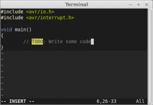 Now that I knew what hardware I had to work with, it was time to start writing the firmware, but before I could get started I needed to decide what would be done with the hardware peripherals, and what would be done purely in software.
Looking at the requirements, I could arrange them in the following order of priority:
- The highest priority was to capture the timestamps of the rising edges of the pulses from each of the four sensors. Positional accuracy comes directly from the ability to accurately measure the difference between these timestamps.
- The next priority was to be able to measure the width of the pulses, so that I could differentiate between the sweeps. Which meant I also needed to timestamp the falling edges of the pulses, but this didn’t need to be so accurate, as the pulse widths differ by about 10us.
- Once the timing and widths of the pulses were measured, the angles would need calculating, and the positions would need to be triangulated.
- Once the positions were known, they would need to be written out to the serial port
Ideally I would have been able to use hardware timer capture units to capture both the rising and falling edges of the pulses, which would have provided all the information needed for requirements one and two. Unfortunately the ATmega3209 doesn’t have eight timer capture units, it’s only got four, and while these are a lot more configurable than the older AVR timers, I couldn’t see a way to make them capture both the rising and falling edges of the pulses and still be able to measure the spacing between them.
However, with four timer capture units, I could at least timestamp the rising edges with no delay, so the most important item on the list would have the best possible accuracy. I could then use pin change interrupts and capture the timestamps of the falling edges in the interrupt handlers. These timestamps would be off by the variable amount of time it would take to get into the interrupt handler, but should be accurate enough.
With the timestamps being collected by hardware and interrupt handlers, I then planned to have the main program loop polling for new timestamps, calculating the widths of the pulses and the distance between them, and processing them to get the angles and positions.
Fine Tuning Timestamp Capture
The plan worked great with one photo diode connected, but connecting two made it a little unreliable, three made it totally fail, and four wasn’t even worth trying.
I had eight interrupt handlers in total, four to store the rising edge timestamps from the capture units, and another four pin change interrupts to read the timers and store the falling edge timestamps. I suspected that these might be taking to much time, so to see what was going on I updated the interrupt handlers so that they would toggle a couple of spare output pins, making them high while in the interrupt handler and low while not. I could then look at how much time was spent in the handlers, and when.
The first thing that I could see was a chain of four pulses showing the time in the timer capture handlers, and that going through this chain took more time than the width of a sync pulse. That meant that with all four sensors triggering a capture interrupt, the pin change interrupt to grab the falling edge was delayed too much to get a meaningful timestamp.
The amount of time I needed to save here wasn’t all that much, so I decided to try eliminating as much of the interrupt overhead as possible, and I declared these interrupts as ISR_NAKED, so that the compiler wouldn’t generate all the entry and exit code to save and restore registers, and I wrote my own minimal handler in assembly.
This worked, and cut the time in the rise handlers in half, and they would complete with time to spare before the sync pulses fell. Now two sensors worked perfectly… but three was a bit unreliable, and four still failed completely, but at least it was progress!
Now the problem was the pin change interrupts for the falling edges, with one or two of them triggering I could collect timestamps with an acceptable amount of error, but with three or four it just took too long before the last interrupt handler ran, so its timestamp was far too inaccurate. This time simply reducing the overhead wasn’t going to cut it, I needed to lose far too much time for that.
After a lot of thought, the solution came to me… I didn’t need four separate interrupt handlers for the pin change interrupts from the four sensors. I had each sensor connected to pin 0 on banks B, C, D and E, and I was routing these pins to the four timers and setting up four pin change interrupts on the same pins.
If I split the signals from the sensors, so each one went to two separate pins, then I could have all the pin change interrupts on one bank, with one interrupt handler. Additionally, in the handler I could grab the timestamp on entry and then check all four pins, regardless of which one actually triggered, and clear the interrupt flags so that it wouldn’t come back in for the other pins. That way, a lot of the time, I would only enter the handler once for all four sensors, instantly cutting my overhead to a quarter of what it was.
Lighthouse Differentiation
 Up until this point, I’d only been working with one lighthouse, mostly just because I hadn’t got around to unscrewing the second one a bringing it upstairs to the workbench. Now that I had reliable capture of all of the pulses, it was time to try adding another one.
First, I wanted to check that I really could handle all the pulses, even with both lighthouses running, which luckily I could. Secondly, I wanted to work on differentiating them, which turned out to be a bit trickier than I first imagined.
On the face of it, it seems fairly simple, the master lighthouse is the first synchronisation pulse, and the slave is the second. But what happens if the master is out of sight, then how do we tell that the slave is the slave? When the master isn’t visible, the slave is the first pulse, but I don’t want to get them confused as the position information will go crazy if I start saying that the master has the angles from the slave.
The solution that I settled on was to use the time since the start of the cycle, not the pulse count. Unlike counting pulses, where I can only have as many as there are visible lighthouses, when using the time since the start of the cycle, I can fake the start time by adding 8333uS to the last one, even when no lighthouses are visible at all.
Then, if there is a pulse approximately around 400uS since the start of the cycle, it’s the slave, otherwise it’s the master (or it’s so out of whack that I might as well start again and consider it the master). When one or both of the lighthouses are visible, I can use them to update the cycle start time to account for any drift between the microcontroller clock and the lighthouse clock. When none are visible I can fake it, and then even if the slave becomes visible again before the master, I can still recognise it as the slave as it’ll be somewhere near the 400uS mark.
Dodgy Timestamps Again

Pulse Widths – 2 Lighthouses
Pulse Widths – 1 Lighthouse
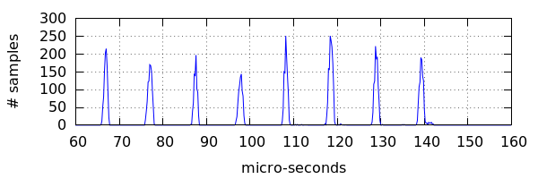
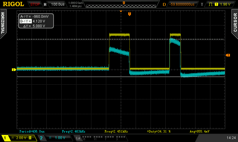
While I was working on the code to differentiate between the lighthouses, I started to see some weirdness with the pulse timestamps again. It was working fine pretty much all the time, but I was occasionally seeing pulses that were too long to be valid. Strangely, it was only happening when both lighthouses were visible. If I blocked the view to the master lighthouse then the timestamps were fine, if I blocked the view to the slave then the timestamps were fine, but if both were visible then I occasionally got a pulse width that was too long.
To get an idea of what was going on, I modified the code to collect the data to create the pulse length distribution graphs shown above. As you can see in the first graph, when only one lighthouse was visible the pulses fell into relatively narrow and symmetrical windows. Then in the second graph, when two lighthouses were visible, the windows started to stretch. This was seen most dramatically in the longest pulses, where instead of having a tall sharp spike in the distribution, I instead got a low, wide, almost square distribution.
Longest Pulse Jitter
This didn’t make much sense, the two lighthouses don’t generate pulses at the same time as each other, and having another lighthouse running couldn’t change the width of the pulses from the other. The problem only occurred when they were both visible to the sensor, they could be visible to each other and the problem wouldn’t happen as long as they weren’t both visible to the sensor.
Pulse Stretched
Pulse Not Stretched
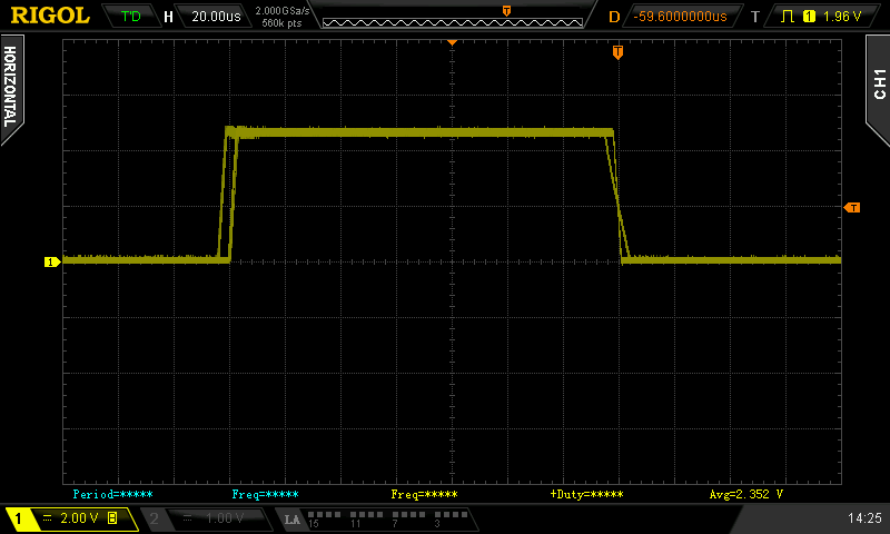
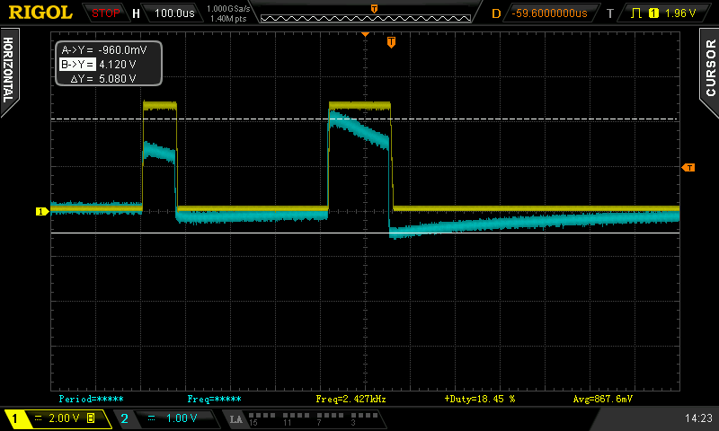
After playing around with the pulse width trigger mode on my ‘scope I was able to narrow down the problem a bit. As the two traces above show, the wide pulses only got stretched when they were preceded by a pulse from the other lighthouse. In these traces the yellow trace is the output of the second op-amp, and the blue trace is the output of the filter before it enters the second op-amp.
I really don’t know what I’m doing when it comes to analogue electronics, but I suspect what is happening is the filter capacitor is still holding some charge from the pulse from the first lighthouse, then the pulse from the second lighthouse adds to this and the input to the second op-amp is much higher than it would have been without the first pulse. Then I think this must be saturating something within the op-amp, which causes the slope of the falling edge to be shallower, widening the pulse.
More Op-Amp Problems
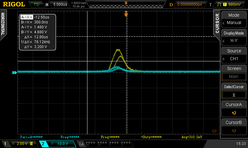
Slow Rise Time
So far, I’d had both lighthouses positioned fairly close to the sensor, just for convenience, but when I tried moving one of the lighthouses to the other side of the room I started to lose pulses and get more bad timestamps. This time is was just down to the rise time of the filtered signal. As the lighthouse gets further away the line it projects sweeps across the sensor faster, and therefore the pulse that the sensor sees gets narrower. When the lighthouse was at the other side of the room, the pulses were narrow enough, and the rise time slow enough, that the output of the amplifier never made it to a high enough voltage before the beam passed and it started falling again, and the microcontroller never saw the pulse.
I could partially fix this problem by raising the cut-off frequency of the filter, and by increasing the gain, but both of these conflicted with the fix for the stretched pulses, and I was unable to fix both issues at the same time. Additionally, increasing the gain was introducing too much noise and was on the verge of creating phantom pulses.
Discrete Photo-Diode Amplifier
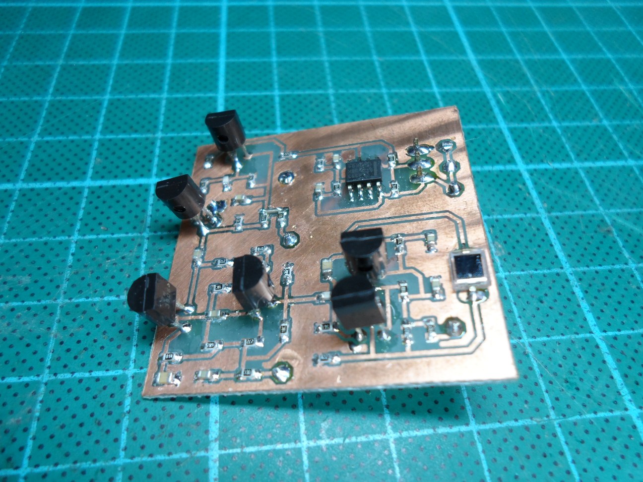
Discrete Photo-Diode Amplifier
As the design obviously worked, I just went ahead and laid out, and etched a PCB. This also didn’t work, but this time I could at least see a viable signal rather than the mountain of noise that I saw on the breadboard. Then with the aid of this SPICE simulation that I could compare signals against, I fairly quickly narrowed the problem down to a missing power supply connection to the envelope detector stage.
With that fixed, it worked great. Much better than the op-amps. Even narrow pulses from the other side of the room rise fast enough to be square, and on top of that the noise rejection is a lot better. While working with the op-amps I hadn’t even noticed that the light from the lighthouses is modulated at 2MHz. The discrete amplifier has a band-pass filter stage that rejects everything that isn’t modulated, so short of completely saturating the diode, there are no worries about varying background light levels.
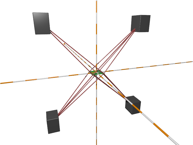
Solving Lighthouse Position & Orientation
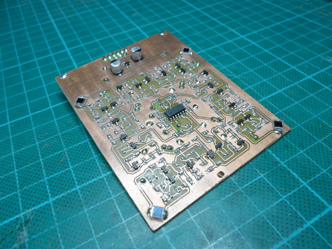
Four Discrete Amplifiers
I wasn’t expecting to have to do much here. Someone else had been here before me, documented their work, and provided a python script to calculate the position of the lighthouses when given the angles to four photo-diodes that are arranged in a square grid.
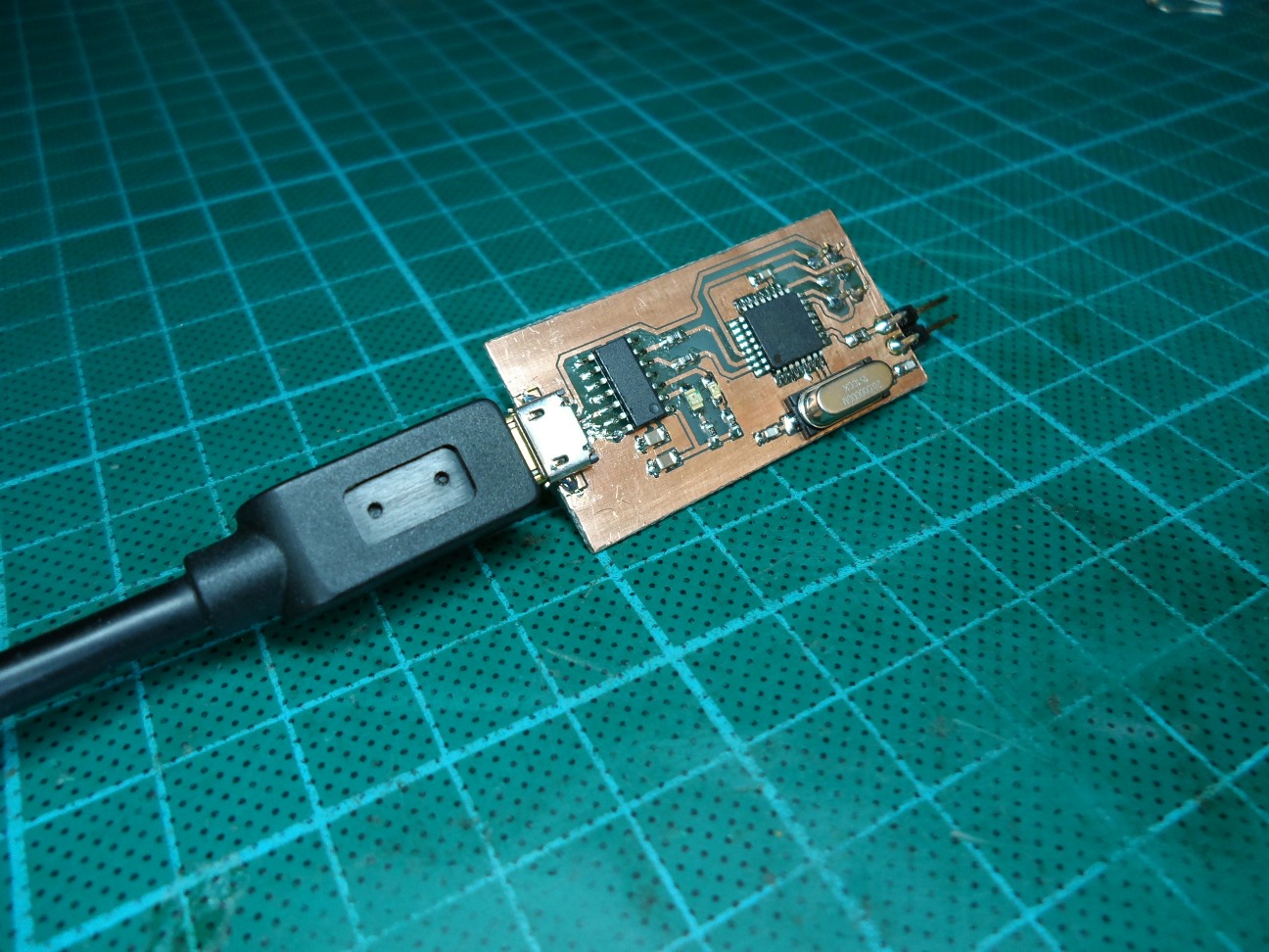
So I laid out a new PCB that contained four photo-diodes and four copies of the discrete amplifier, etched it, and then spent a couple of evenings painstakingly soldering a couple of hundred components to it. Surprisingly there were no mistakes and all four sensors gave a good signal straight away, so thinking I was only a few minutes away from calculating an actual position, I fed the data to the python script…
The script promptly output the X, Y, and Z coordinates of the four sensors, but that wasn’t what I needed! I needed the coordinates of the two lighthouses, and I also needed a matrix of nine numbers for each, describing the rotation. Hmm… how on earth was I supposed to get the lighthouse position and orientation from this?
I hunted high and low in that repository. I could see that the firmware contained a hard-coded structure that held the position and rotation matrices that I needed, and I could see the solver script that only gave me the sensor positions, but nowhere could I find the missing piece that would get from one to the other.
Apparently I wasn’t going to get away with avoiding actually understanding the maths, which was bad, because I’m terrible at maths. The only bit of trigonometry that I can actually remember is a2 + b2 = c2!
Finding A Common Point Of Reference
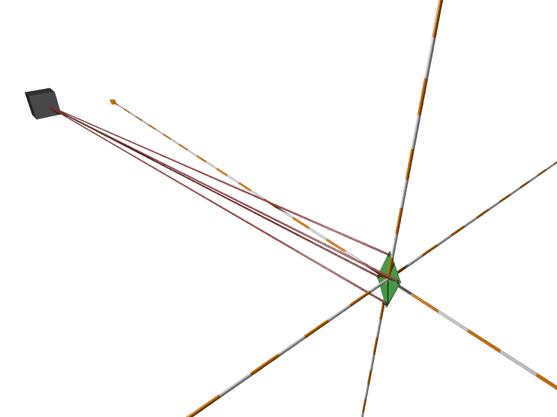
Sensors At Origin
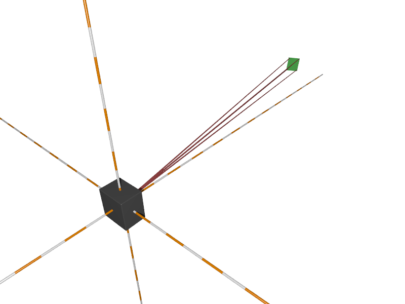
Lighthouse At Origin
That wasn’t much use on its own though. The master lighthouse was at the origin, but so was the slave, just in two totally different coordinate systems. What I needed was a common point of reference. I needed the position of the lighthouses relative to the sensors. I could do that with a simple translation. If I calculated the center of the sensor plane (subtract the vector of one corner from the one diagonally opposite and divide by two), then I could move it to the origin by subtracting the resulting vector from each of the sensor points, and I could move the lighthouse by the same amount, moving it away from the origin.
That gave me the coordinates of the lighthouses relative to the sensors, but there were two related problems remaining. I still didn’t know the rotation of each lighthouse, and the coordinates of the two lighthouses still weren’t actually in the same coordinate system. Although the sensor plane was now centered at the origin from the point of view of both lighthouses, I didn’t know what angle it was at, and that angle would be different for each lighthouse.

Complete Solution
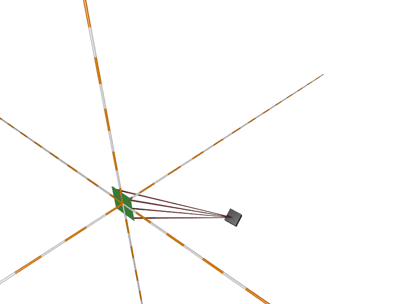
Common Rotation Reference
To do this I calculated the normal vector of the sensor plane (the vector perpendicular to the plane), and then calculated the rotation matrix that would align it with the Z axis. Then I calculated the rotation matrix that would align the edge of the plane that connects sensors 0 and 1 with the Y axis. I’ve no idea how the maths to calculate these rotation matrices works, but luckily Google came to the rescue and gave me a handy function to calculate a rotation matrix when given two vectors that need aligning.
Applying these rotation matrices to the sensor points and the lighthouse swung everything into a known orientation, and now instead of having the lighthouse aligned with the axes, and the sensors at an angle, I had the sensors aligned with the axes, and the lighthouse at an angle. I could also multiply the two rotation matrices together to get the final rotation matrix that I needed to describe the lighthouse orientation. Then I just needed to repeat for the other lighthouse, and I had the complete solution. I had the position and orientation of both lighthouses, all in a common coordinate system, ready to use for triangulating positions.
Triangulating Positions
Now that I had the lighthouse solution that I needed, I could finally implement the last step and triangulate the position of a sensor from the angles to it from the two lighthouses. The process is fairly straightforward, but there is a complication that arises when extending triangulation from 2D to 3D.
Working the problem on a piece of paper in 2D, you draw a line from the first lighthouse at the first angle, then you draw a line from the second lighthouse at the second angle, and where they meet is the position of the sensor. In 2D, unless the lines are parallel, they will always meet. What wasn’t immediately obvious to me, was that in 3D, this isn’t the case. In fact, in practice the lines are never actually going to meet. It only takes the tiniest error in one of the angles to nudge one of the lines off course so that it will pass over, under, or to the side of the other line.
To get around this problem we don’t calculate the intersection of the lines, instead we calculate the nearest point between the two lines. Once again, I don’t really understand how that calculation works, but luckily I get to borrow the function that does it from the people that have been here before me.
A quick copy and paste, and… it works! I now had positions, in millimetres, being streamed out of the serial port, and pushing the sensor around the bench was changing the numbers by a plausible amount.
More Stable Solver & Applying Gravity
While I was cleaning up the code after getting everything working, it quickly became apparent that there was a problem. The non-linear equation solver that computes the distances of the sensors from the lighthouse was not always finding a usable solution. In fact it was failing more often than not. If one edge of the sensor board was roughly square to the lighthouse then it would always find a solution, but as the board was rotated, and the angle of the edge increased, it would start failing, and it would continue failing until the next edge squared up to the lighthouse.
That part of the solver script was still unmodified from the trmm.net version, which was using the nsolve function from sympy. I didn’t like that this was essentially a black-box, with very little description of what goes on inside, and how it actually solves the system of equations, so I started to look around for alternatives. One of the alternatives that I found was scipy.optimize.leastsq, which I was attracted to because I had at least a vague idea of what Least Squares was.
As luck would have it, plugging in this alternative solver made an immediate improvement. It was finding a good solution almost all the time. After some playing around I tried adding an extra equation that would make it prefer solutions where the distances to the sensors differed by less than the grid size, and this seemed to make it even better, with it becoming difficult to find cases where it would fail to find a solution.
The last tweak that I made to the Python solver was to get it to rotate the entire solution to account for gravity. The lighthouses contain accelerometers, and broadcast a vector in the OOTX data that tells us which way is down. It was a simple modification to collect these vectors from the broadcast data, average the vectors from each lighthouse together, and then calculate and apply a rotation matrix to bring the solution into line with gravity.
Making It Standalone
This is where I should have been done, but the whole time I’d been working on this it had been bugging me that I needed to offload the initial lighthouse solution to another processor. It just seemed like such an ugly solution… if only it was possible to implement the solver on the AVR CPU…
Moving to Least Squares had been a good start, I knew that I needed to implement a non-linear least squares solver, and that gave me a starting point for some research. A bit of time with Google revealed that numerous algorithms existed, but the core algorithm behind a lot of them was the Gauss-Newton method, so that seemed like a good place to start. Now I just needed to get enough of an understanding of it to be able to implement it in C.
If I’m understanding how it works correctly, then it goes something like this:
- Start with an estimate (or wild guess) of the unknown variables
- Calculate lines that match the slope of the non-linear function at the point indicated by the current estimate of the unknown variables
- Use a linear solver to follow the lines and find a new estimate for the unknowns
- Repeat steps 2 and 3 to keep following the curve of the non-linear function until we get stuck in a minimum, which is hopefully the solution that we were after
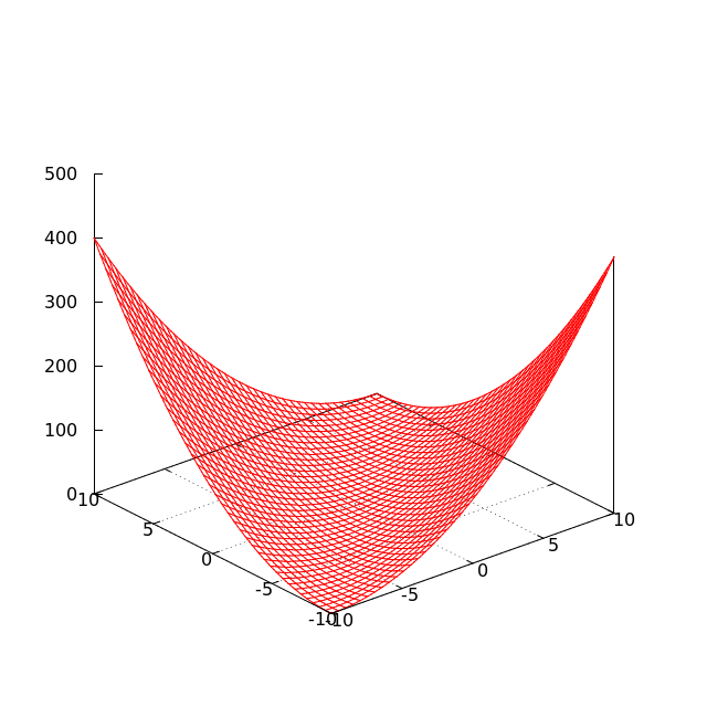
Non-Linear Function
The set of non-linear equations that I’m using are the same ones used in the Python solver, that were derived by trmm.net. It’s easy to see that all six are essentially identical. The unknown variables and the constants change, but the overall function is the same. I wrapped this up in a function:
scalar_t residual(scalar_t a, scalar_t b,
                  scalar_t c, scalar_t d)
{
        return a*a + b*b - 2*a*b*c - d*d;
}
The function is called residual as its purpose is to return the error when using the current estimates of the unknown variables. It is returning how far away we are from having the equation equal zero.
From the steps of the Gauss-Newton method outlined above, I needed to compute a set of linear equations that describe the slope of these non-linear equations. This is done using a Jacobian Matrix, which is just a table that has one row for each of our six equations, and one column for each of the four unknown variables. The values in the table are the results from feeding the current estimate of the unknown variables to the partial derivatives of our non-linear equations.
So for example, row one represents equation one, and in that row, the value in column one comes from the partial derivative of that equation with respect to the first unknown variable, the value in column two comes from the partial derivative with respect to the second variable, and so on.
It turns out that not only are all six of the non-linear equations essentially identical, but so are all of the partial derivative equations, which I wrapped up in this function:
scalar_t partial(scalar_t a, scalar_t b, scalar_t c)
{
        return 2*(a - b*c);
}
Working out the partial derivative equations involves following a magic set of rules. I’m sure there’s some logic behind them, but it escapes me. Alternatively, this handy derivative calculator website will do it automatically.
With the Jacobian matrix populated, the next step was to solve the set of linear equations that it represents. This I did using another bit of black-box mathematical magic like so:
- Multiply the Jacobian matrix with a transposed version of the same matrix, which results in a square, invertable matrix (transposed means rotated on its side, so the rows are the columns and the columns are the rows)
- Calculate the inverse of the resulting matrix
- Multiply the inverted matrix with the transposed Jacobian matrix again, which gets us back to a 6×4 matrix
- Multiply that with a 6×1 matrix of the residuals from the non-linear equations
The result of solving the linear equations is a set of four values, which give the amount that the estimate of each unknown should be adjusted by. Then once the estimates have been adjusted it’s just a case of looping, building a new set of residuals and a new Jacobian matrix using the new estimates, and repeating until we’re adjusting the estimate by such a small amount that it’s not worth continuing.
The only real surprise when implementing this in C was what is hiding behind the little -1 that indicates an inverted matrix on the Wikipedia page. Inverting a 4×4 matrix requires somewhere in the region of 200 multiplies! I would guess that this is consuming the majority of the processing time of the whole solver.
Quite often it only takes this solver around five iterations to find the solution, which it manages to do in around 100 milliseconds. It also only uses around 500 bytes of memory, so in the end it turned out to be well within the capabilities of a little 8-bit micro-controller.
Detecting & Fixing Bad Solutions
Multiple Solutions
It turns out that having the sensors on a flat plane isn’t actually a good idea. When they’re on a plane there isn’t just one solution for the solver to find. There are at least four solutions (that I’ve found so far), and only one of them is useful to us.
Those possible solutions are:
- The one we want, the sensor board is in front of and below the lighthouse. A beam projects from the front of the lighthouse and hits the top of the sensors.
- There’s another where the sensor board is above the lighthouse, and a beam projected from the lighthouse passes through the sensor board and into the bottom of the sensors. impossible in real-life, but a mathematically valid solution
- Another possibility has the sensor board behind and below the lighthouse, with the solver giving us negative distances to the sensors. A beam projects out the back of the lighthouse and hits the top of the sensors.
- Finally, there’s a combination of solutions (2) and (3), where the sensor board is both behind the lighthouse and above it, with a beam projecting out the back of the lighthouse and through the bottom of the sensor board.
The solutions where the sensors are behind the lighthouse are very easy to detect, just look to see if the distances returned by the solver are negative. The solutions where the board is above the lighthouse were harder to detect, in part because the lighthouse could be in any orientation, it’s perfectly valid to mount one upside down or on its side.
Luckily, I had the accelerometer data from each lighthouse. I could calculate the normal vector of the sensor plane as seen by the lighthouse, then compare that vector to the gravity direction vector from the lighthouse. This then told me if the sensor plane was above the lighthouse, in which case I could just flip the distances around to get the correct solution.
It’s Done!
With the invalid solutions being rejected, I think I’m finally done. Now whether the lighthouses are nearby or far away, as long as all the sensors can see both lighthouses, I always seem to get a valid usable solution within a few seconds.
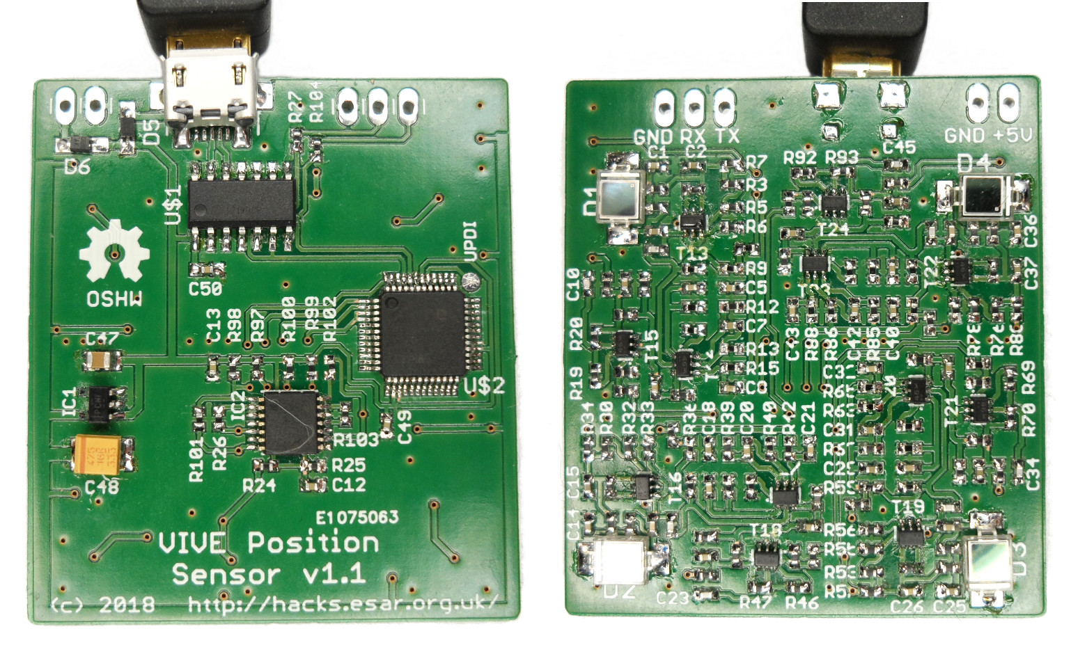
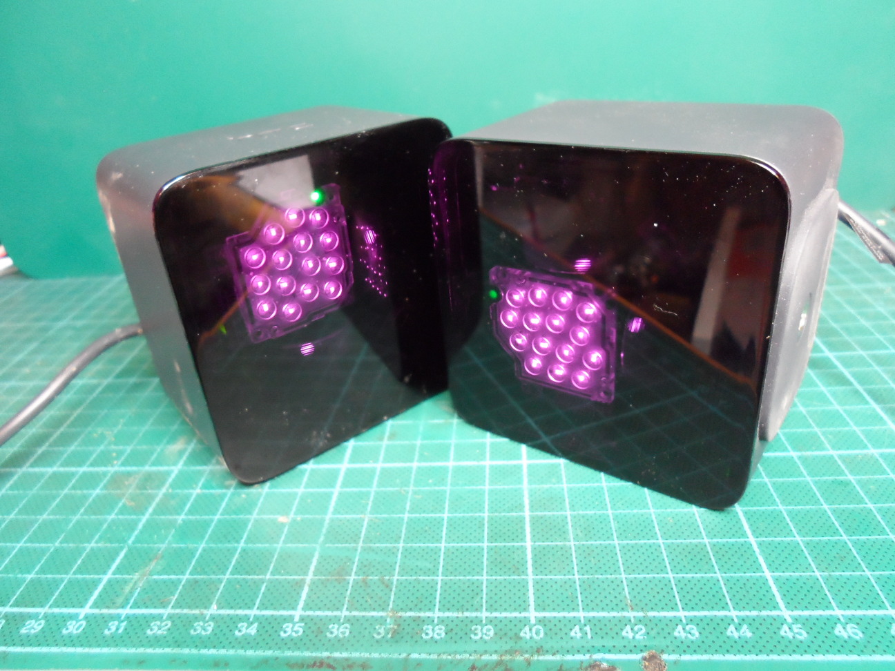
The board shown at the top of this page is the final result of all of this work, and can be found, along with the firmware, in my github repository. Simply connect a USB cable and it will appear as a serial port, and it will start streaming out position data as soon as it works out the position of the lighthouses.
As well as the position data, the board also constantly streams out several other pieces of information:
- The raw angle tick counts from each sensor
- The OOTX data from each lighthouse
- The position and orientation of each lighthouse
- Various status messages
All of the data is in a simple text format and the included solve-lighthouse.py script can be used to filter and format the data. This script also includes the old python solver, though this is now out of date and should probably be ignored.
To output the position data from sensor 0, simply run (changing /dev/ttyACM0 to match the name of the serial port on your machine):
solve-lighthouse.py --dump-pos --dump-sensor=0 /dev/ttyACM0
The output will look like this:
0:    X:   -113.3    Y:   -477.3    Z:   -760.7    err: 0.02
0:    X:   -113.4    Y:   -477.0    Z:   -760.8    err: 0.01
0:    X:   -113.1    Y:   -477.0    Z:   -760.6    err: 0.13
The position data is in millimetres and the origin is the master lighthouse, so multiple sensors can be used and they should agree with each other about their positions.
Bugs & Future Work
Although this is already the second revision of this board, there are still a couple of bugs:
- Most importantly, the power trace from the USB port is only insulated from the body of the USB socket by the solder mask. This trace just needs moving to the other side. If anyone builds this board without modification then it may be worth adding a bit of kapton tape before soldering the socket down, though so far I seem to have gotten away without it on mine.
- The silkscreen labels for the UART pins are wrong. I forgot to rearrange them after I changed the pinout from the v1.0 board.
There are also a couple of changes that I’d like to make to the lighthouse position calculation. At the moment the board will calculate lighthouse solutions repeatedly at power up until it finds one with acceptable error, then it will use that solution until it is power cycled. I’d like to make the following changes:
- Instead of using one solution found at startup, make it calculate several solutions and average them together to get a more accurate position for the lighthouses
- Detect and react to lighthouse position changes. Either by regularly recalculating the position of them, or doing so in reaction to the triangulation error increasing
Looks like an interesting artical.
Sadly i didn’t had the time to read it yet. Maybe next sunday 🙂
But please continue making this types of artical. I especially liked you HDMI ambient light stuff because of the FPGAs <3.
it’s cool
Congratulations Stephen very few people have ever got poses out of raw Lighthouse data and even fewer have built their own tracked objects including analogue front ends and got it all working. Lighthouse has many layers of complexity and trust me I know getting poses even without calibration correction is a lot of work!
If you are ever curious about Lighthouse again and want to ask questions I am happy to answer them. Lighthouse 2.0 is an even bigger challenge as it has no global sync pulses and sync needs to be recovered from the modulation on the swept laser beams. Also the geometry of the single rotor scanner is a lot more complex mathematically to solve.
Thanks Alan. While it was way more work than I expected when I started, it had me hooked, and I had a lot of fun solving it. I’m still slowly making progress on the project that needed the position data, and with a bit of luck it may even appear here before the end of the year.
I’ve not been following what you guys have been up to recently, but the 2.0 lighthouses sound intriguing, I’ll have to go do some reading.
Wow this is exactly the resource I’ve been dreaming about! I’m late to the game it being 2023 now but I got an HTC Vive headset recently and it inspired me to create something like this. As I’m writing this, I’ve got the infrared sensors and TS4231 chip plus custom PCB on the way. I’m opting to go for an FPGA right now so starting with an Upduino with an ICE40 so it’ll be a new learning experience for me. I’d love to pick your brain once I get rolling!